Tunnel Exploration PDFS
In the field of autonomous mobile robot navigation within tunnel environments, complex structures, and dynamic challenges require specialized exploration strategies. Although conventional methods like depth-first search offer insights in graph-like scenarios they may not fully address the intricacies of tunnel networks. Herein lies the solution: Priority-Based Depth-First Search (PDFS), a customized exploration strategy that can maximize tunnel exploration and simplify the data collection process. Particular difficulties seen in tunnel environments include branching paths and interconnected junctions, necessitating exploration strategies that adapt to these complexities. With an emphasis on critical places inside the tunnel structure, PDFS is designed specifically to prioritize exploration in order to navigate such situations efficiently. PDFS strategically prioritizes exploration according to predetermined criteria and acknowledges the importance of branching pathways within tunnel networks. Through prioritizing vital regions, PDFS guarantees a more focused and effective research procedure.
PDFS dynamically modifies its exploration trajectory to conform to the complex structures of tunnel environments by using a depth-first strategy. Because of its flexibility, the algorithm can efficiently explore a wide range of combinations and find its way through complex pathways. Real-time decision-making processes are incorporated into PDFS so that the algorithm can adjust to shifting environmental conditions. When faced with unexpected challenges or dead ends, PDFS can quickly modify its research plan to increase efficacy and efficiency.
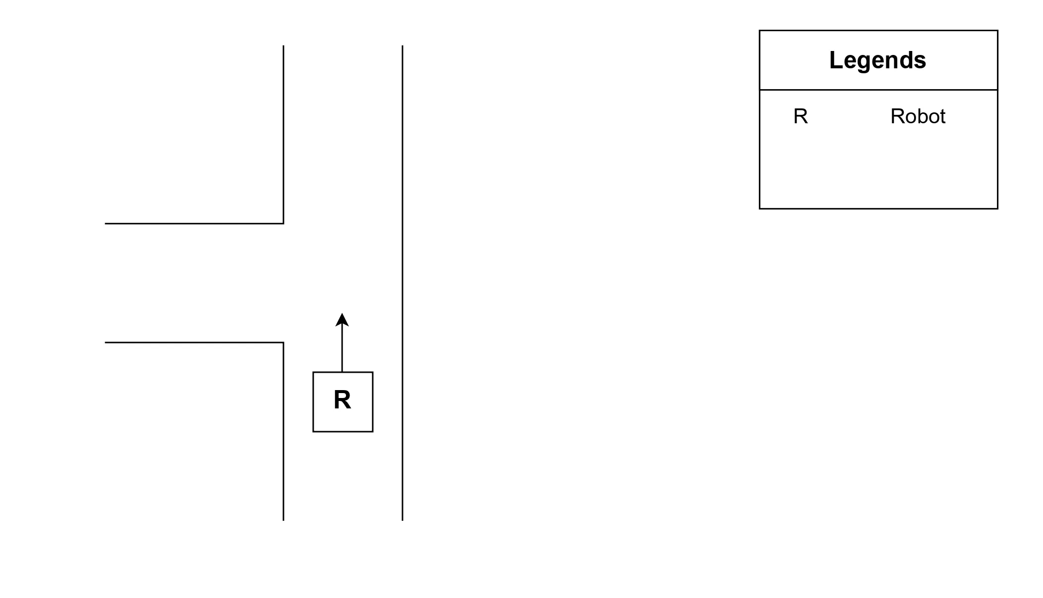
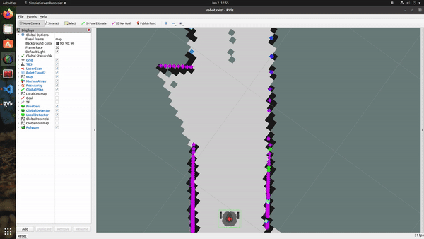
Priority-based Depth First Search is the heart of the exploration algorithm as it helps the robot to navigate in case of a junction detection by sending F1 as the next potential frontier to be explored and also in case of a dead-end detection. PDFS keeps track of all the junctions detected and provides the next potential frontier for further exploration.
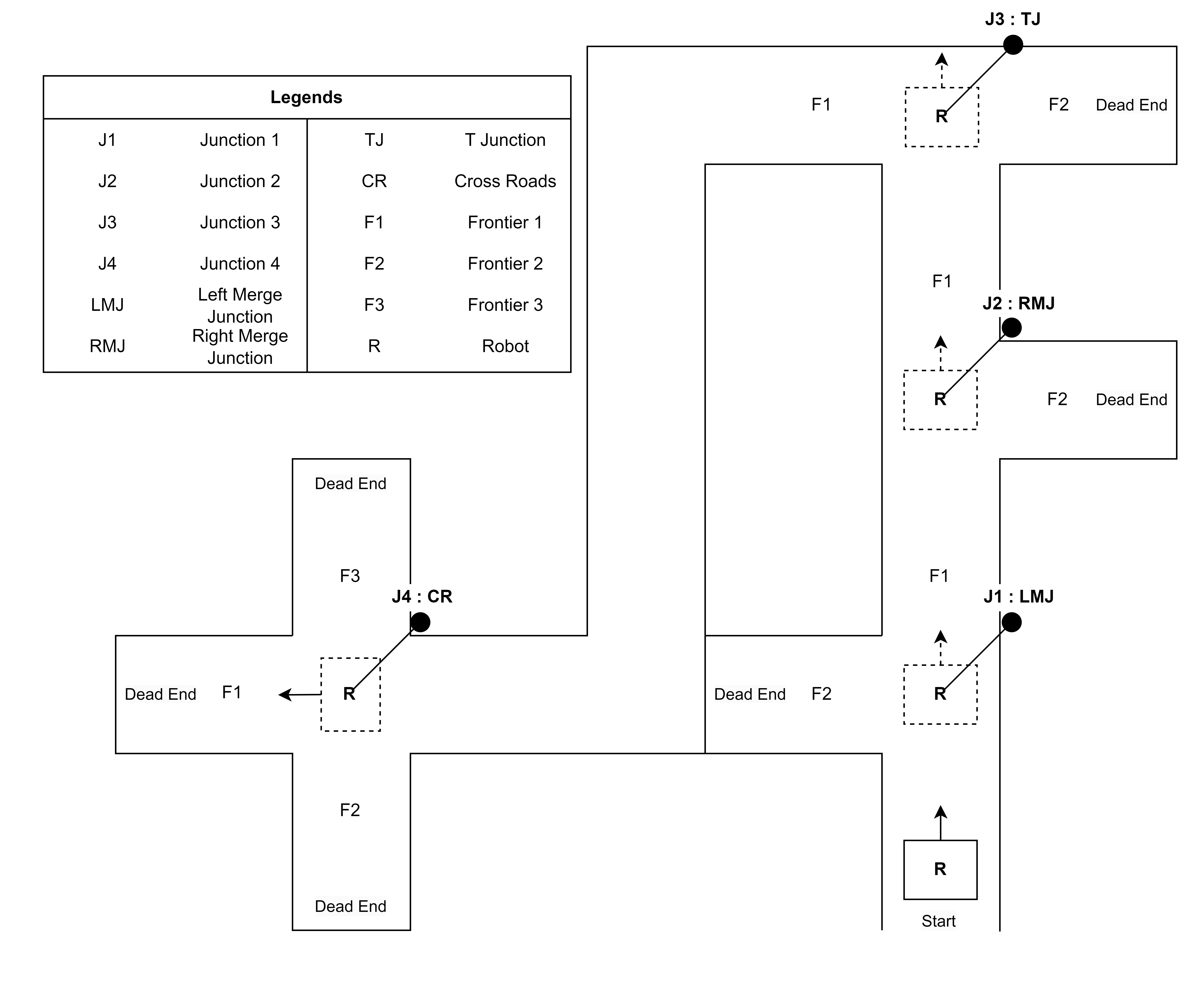
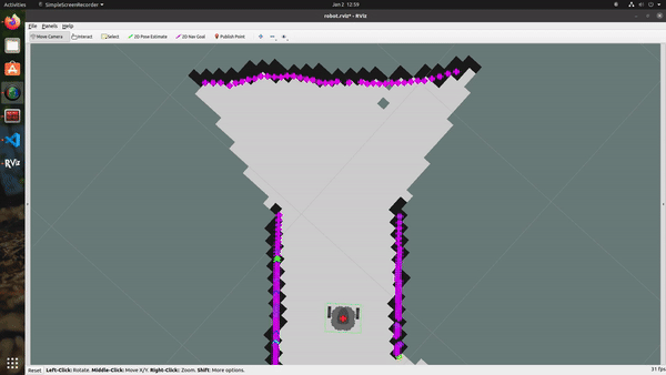
1a. Priority Based Depth First Search Map.
The Fig. 1a illustrates the working of a PDFS algorithm in an environment.
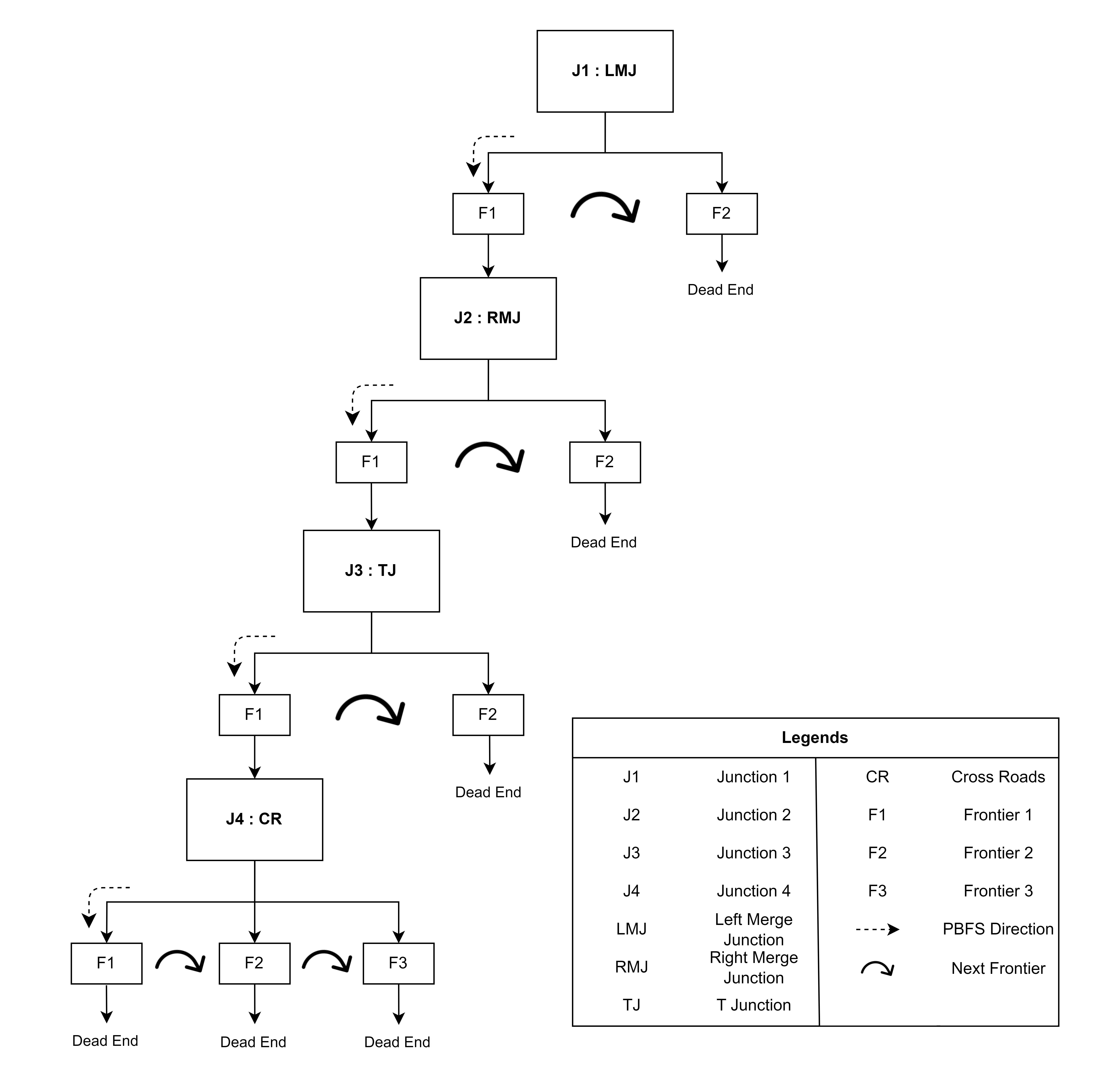
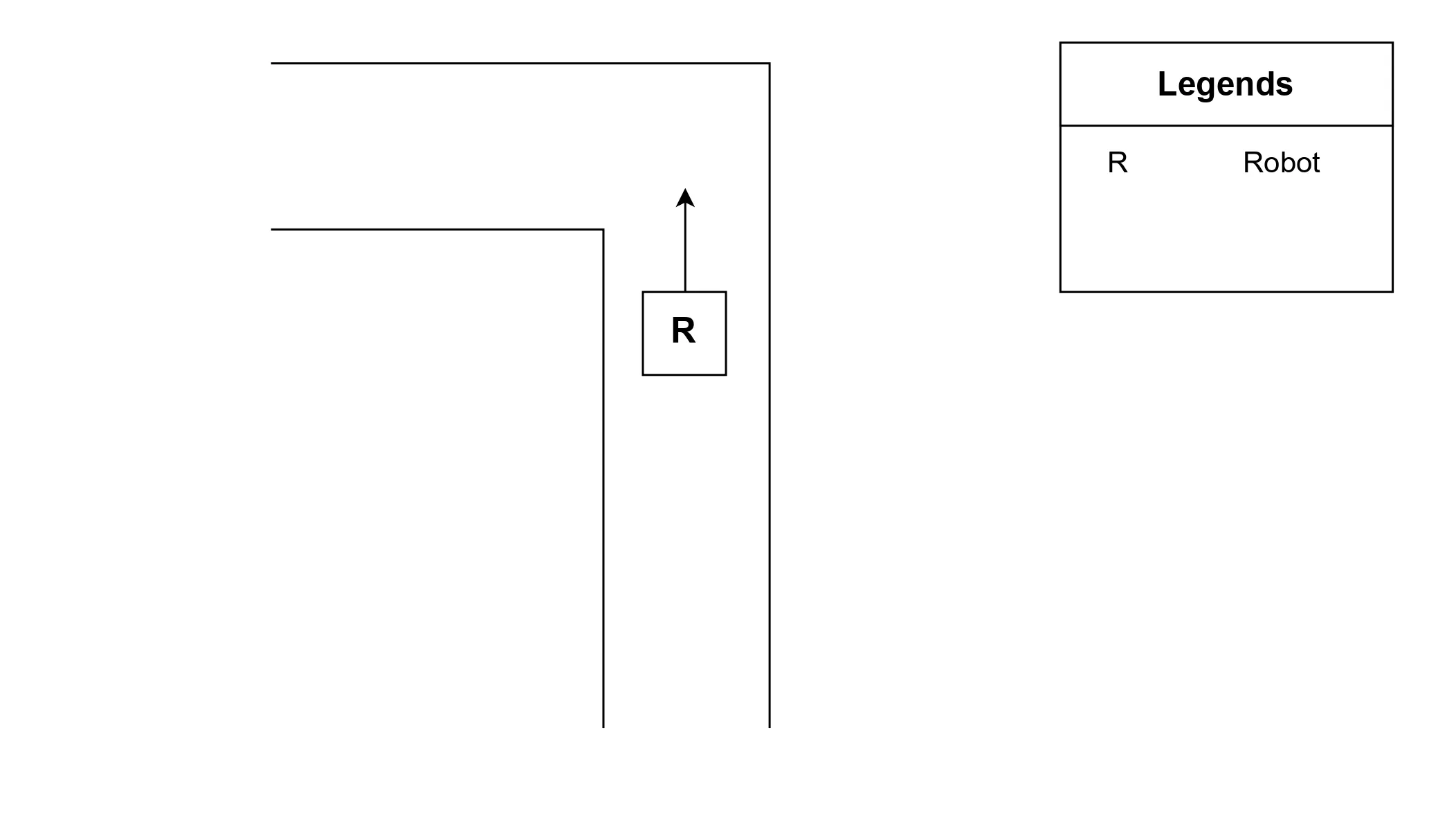
PDFS gets the information of a junction detected and its frontiers from the junction detector node and maintains a dictionary of junctions and their frontiers containing the inform4f. Frontiers Calculation in Dead Endation on explored and unexplored frontiers. It keeps track of the explored and unexplored frontiers of each junction. For example, it always continues the exploration in the F1 direction and in case of a dead end, it starts exploring the other unexplored frontiers of the current junction. When all the frontiers of the current junction are explored, it navigates the robot toward the previous junction’s unexplored frontiers. Once all the frontiers get explored it finishes exploration. The Fig. 1b shows an example of pdfs working in the map shown in 1a.
1b. Priority Based Depth First Search Map.
Concluding, the implementation of a Priority-Based Depth-First Search has the potential to significantly transform tunnel exploration tactics by providing customized solutions for efficiently navigating the complexities of tunnel environments. PDFS has the potential to enhance the capabilities of autonomous mobile robot navigation in complex and dynamic tunnel environments by virtue of its strategic prioritization and adaptability.
Development of Approach
A junction is a point where two or more paths/roads intersect or meet. Tunnel structures usually consist of multiple different types of junctions. For effective and prioritized exploration, a large-scale tunnel network itself highlights the importance of the identification of a junction and its type. To identify a junction it is very necessary to understand the structure of each junction.
Junction Types
Following are some common junctions that are commonly encountered during robotic tunnel inspection.
Special Cases
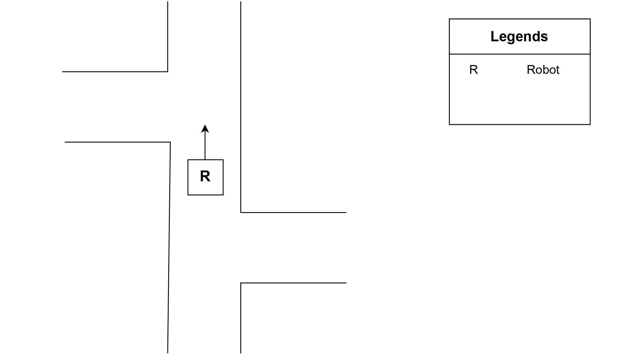
Cross Road Junction
The crossroad junction is the most common junction which we come across in our daily life. It is formed with the intersection of two perpendicular roads. It is also known as a four-way intersection. The Fig. 2a shows an example of a crossroad junction.
2a. Crossroad Junction
T-Junction
T junction is formed when a road terminates into another at a perpendicular angle forming a ‘T’ shape. It is also called a three-way intersection. The Fig. 2b depicts an example of a T junction.
2b .T-Junction
Y Junction
Y junction is the result of a road splitting into two forming a ‘Y’ shape. While these two roads can branch off at different angles. The Fig. 2c is a visual example of a Y junction.
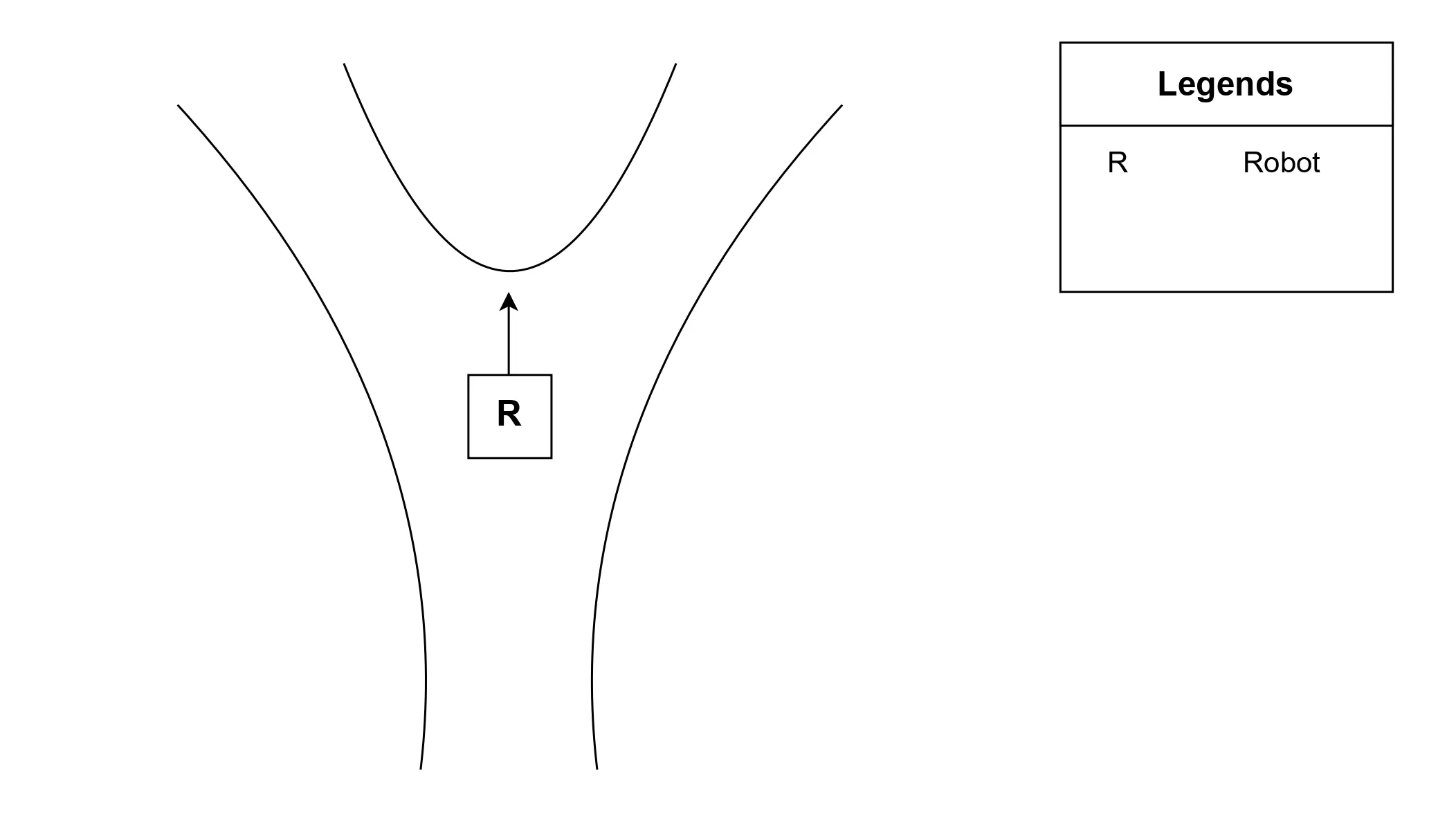
2c. Y-Junction
Staggered Junction
A staggered junction involves two crossroads placed diagonally across from each other with an offset. The Fig. 2d is a good example of a staggered junction. It can be further divided into two types named right merge junction and left merge junction.
2d. Staggered Junction
Right Merge Junction
In a right merge junction, a road from the right side merges into the main road at a 0-degree angle. The Fig. 2e illustrates a right merge junction.
2e. Right Merge Junction
Left Merge Junction
In a left merge junction, a road from the left side merges into the main road at a 180-degree angle. The Fig. 2f illustrates a left merge junction.
2f. Left Merge Junction
Normal Cases
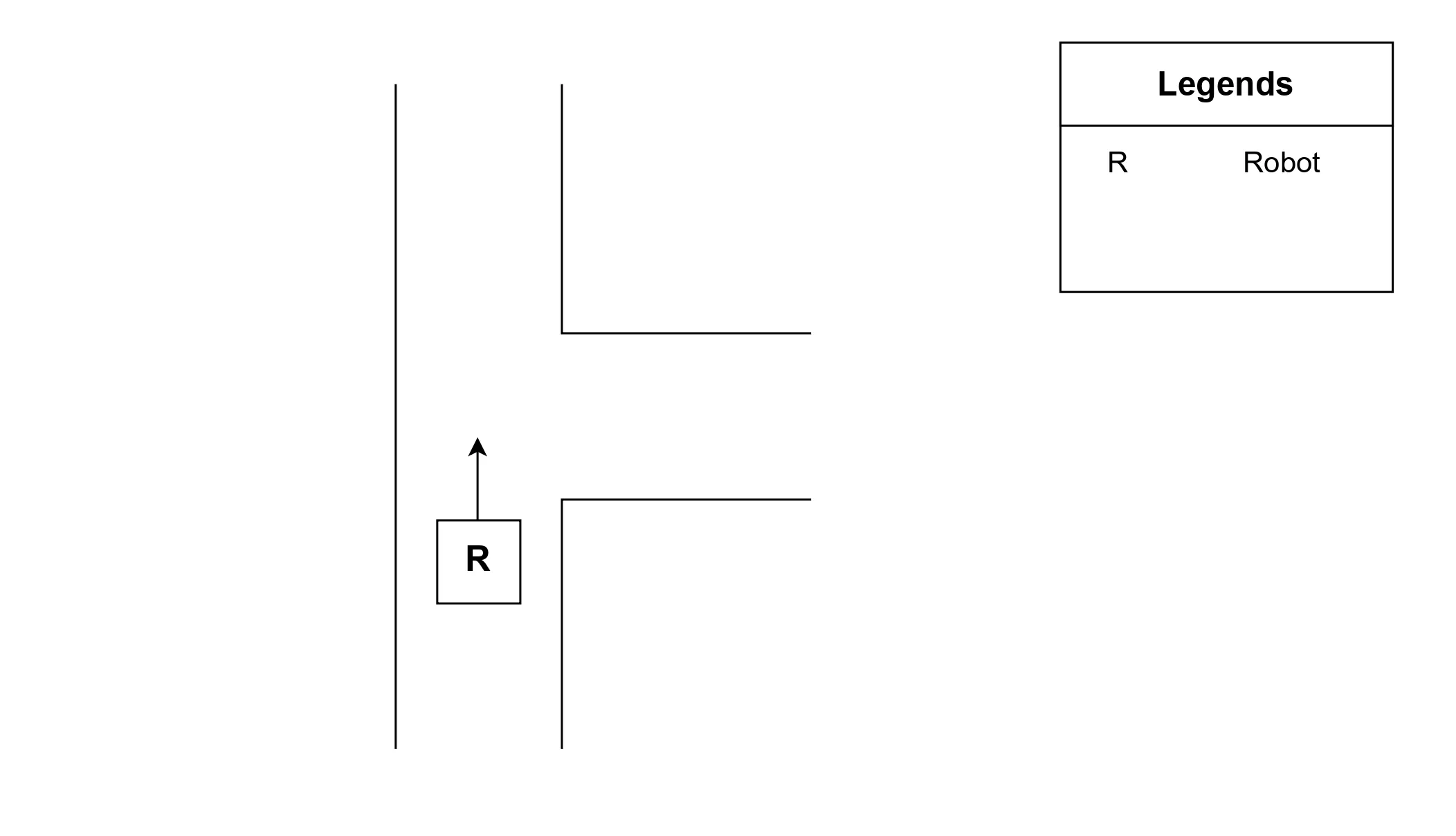
Left Branch
A left branch is a path where a straight path ends and the road turns into a left branch. The Fig. 2g portrays a left branch.
2g. Left Branch
Right Branch
A right branch is a path where a straight path ends and the road turns into a right branch. The Fig. 2h represents a right branch.
2h. Right Branch
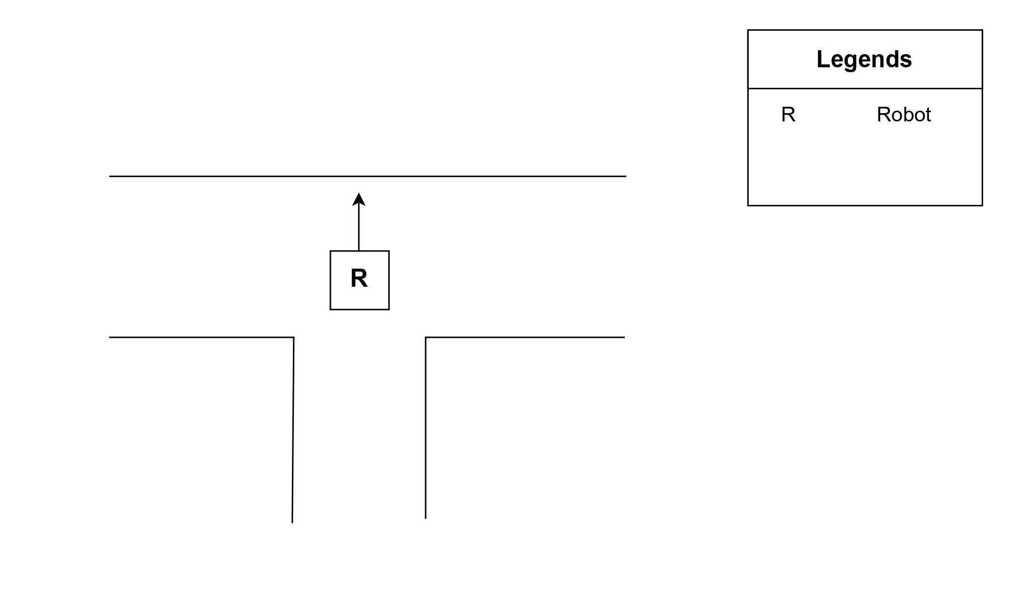
Dead End
In a dead end, the road ends with no other paths except on the back. The Fig. 2i displays a dead end.
2i. Dead End
Straight Path
A straight path is a linear or uninterrupted course that does not involve any branch or junction. The Fig. 2j exhibits a straight path.
2j. Straight Path
Considering the geometry and shape of each junction and robotic coordinate system which is different from the Cartesian coordinate system (as it has a positive x-axis on the vertical front and a positive y-axis on the horizontal left) a technique needed to be developed that could be the most suitable with the structure of junctions to extract most relevant data points. This gave birth to the idea of creating a junction synthesizer.
Environment Segmentation
The purpose of designing a junction synthesizer was to form the area around the robot into a shape that could fit most into the shape of different junction types and retrieve maximum unique and finely categorized data points. Initially, the area around the robot was categorized into 8 different regions named Front(F), Back(B), Left(L), Right(R), Diagonal front left(DFL), Diagonal front right(DFR), Diagonal back left(DBL) and Diagonal back right(DBR). These 8 different sections are named as regions of interest (ROIs). The basic algorithm lies in the precise definition of ROIs. The definitions of ROIs according to their area are given below.
Front (F): Extending in front of the robot in +x-axis direction, filtering points with +x coordinates and -y also +y axis coordinates.
Back (B): Extending on the back of the robot in -x direction, filtering points with -x axis coordinates and -y also +y axis coordinates.
Left (L): Extending on left of the robot in +y direction, filtering points with +y axis coordinates and -x also +x axis coordinates.
Right (R): Extending on the Right of the robot in -y direction, filtering points with -y axis coordinates and -x also +x axis coordinates.
Diagonal Front Left (DFL): Extending towards diagonal left of the robot in the +x direction, filtering points with +x axis coordinates and +y axis coordinates.
Diagonal Front Right (DFR): Extending towards the diagonal right of the robot in the +x direction, filtering points with +x axis coordinates and -y axis coordinates.
Diagonal Back Left (DBL): Extending towards the diagonal left of the robot in the -x direction, filtering points with -x axis coordinates and +y axis coordinates.
Diagonal Back Right (DBR): Extending towards the diagonal right of the robot in the -x direction, filtering points with -x axis coordinates and -y axis coordinates.
Holding the base idea of categorizing the area around the robot into ROIs a few approaches were developed and evaluated according to their design of ROIs.
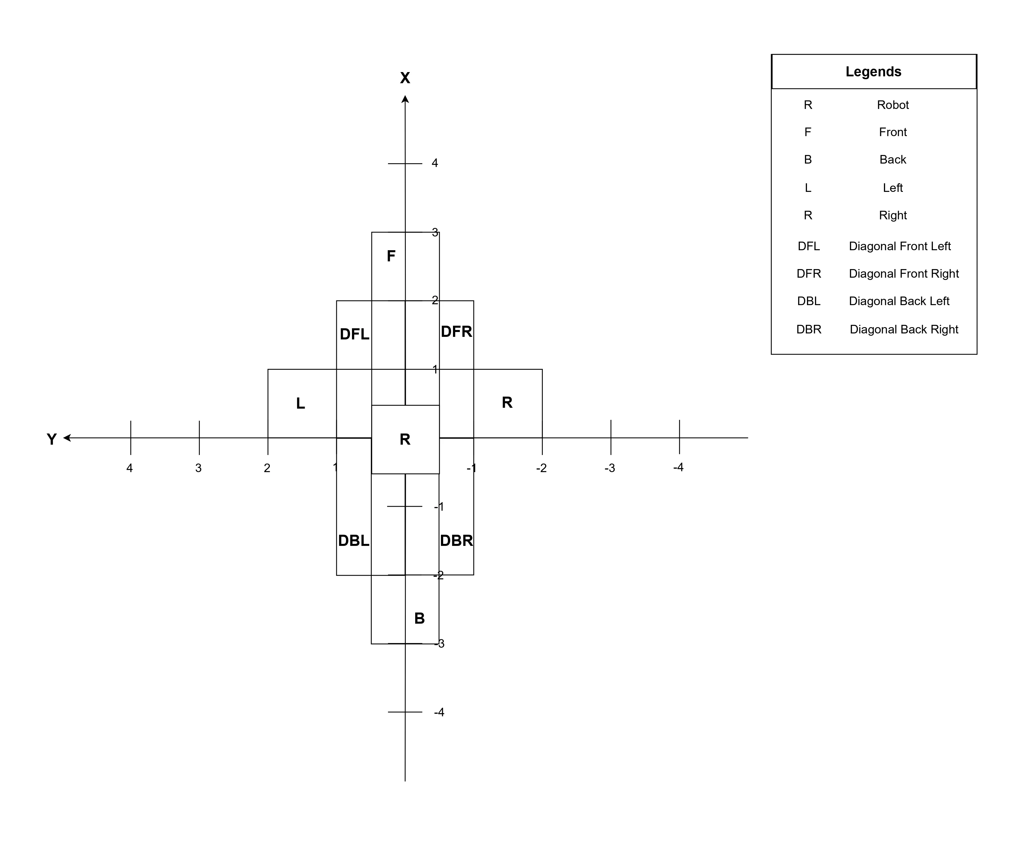
Rectangular Approach
The rectangular approach was designed initially with rough limits. For the rectangular approach, the limits for the corresponding ROIs were as follows:
Front (F): 0m < x < +3m and -0.5m < y < +0.5m
Back (B): -3m < x < 0m and -0.5m < y < +0.5m
Left (L): 0m < x < +1m and 0m < y < +2m
Right (R): 0m < x < +1m and -2m < y < 0m
Diagonal Front Left (DFL): 0m < x < +2m and 0m < y +1m
Diagonal Front Right (DFR): 0m < x < +2m and -1m < y < 0m
Diagonal Back Left (DBL): -2m < x < 0m and 0m < y < 1m
Diagonal Back Right (DBR): -2m < x < 0m and -1m < y < 0m
After applying limits to the corresponding ROIs the rectangular approach design is depicted in the Fig. 3a.
3a. Rectangular Approach
As it is clear from Fig. 3a the regions of interest were not well defined and were overlapping hence the data retrieved was not useful as most of the points were being shared by multiple ROIs at the same time.
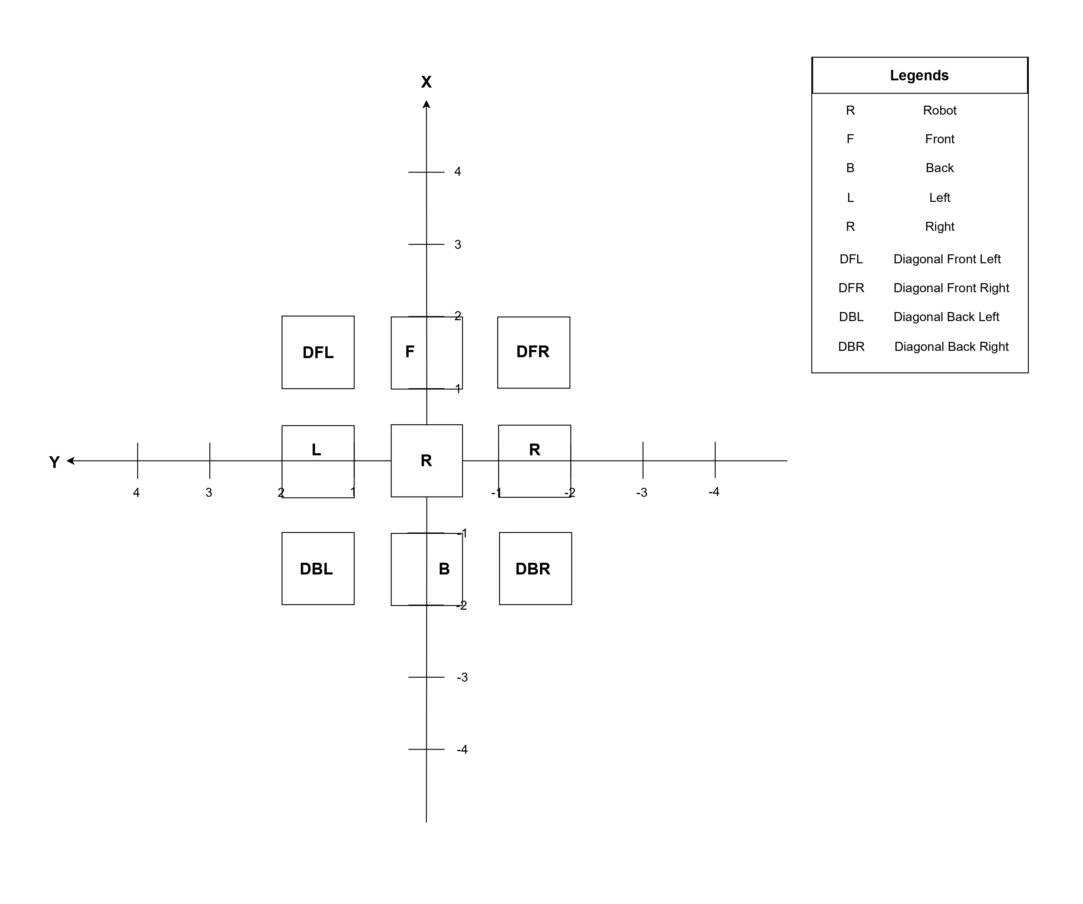
Squared Regions Approach
In the squared regions approach a significant gap was introduced between ROIs and their limits were refined in such a way that each ROI was a square shape. The limit ranges for ROIs were:
Front (F): +1m < x < +2m and -0.5m < y < +0.5m
Back (B): -1m < x < +2m and -0.5m < y < +0.5m
Left (L): -0.5m < x < + 0.5m and +1m < y < +2m
Right (R): -0.5m < x < + 0.5m and -2m < y < -1m
Diagonal Front Left (DFL): +1m < x < + 2m and +1m < y < +2m
Diagonal Front Right (DFR): +1m < x < + 2m and -2m < y < -1m
Diagonal Back Left (DBL): -2m < x < -1m and +1m < y < +2m
Diagonal Back Right (DBR): -2m < x < -1m and -2m < y < -1m
After applying the refined limits the squared region approach design can be seen in Fig. 3b
3b. Squared Regions Approach
As can be seen from the Fig. 3b the limits were well-defined but there were huge gaps between all ROIs which resulted in the loss of most of the data. The rest of the points were not enough to analyze further.
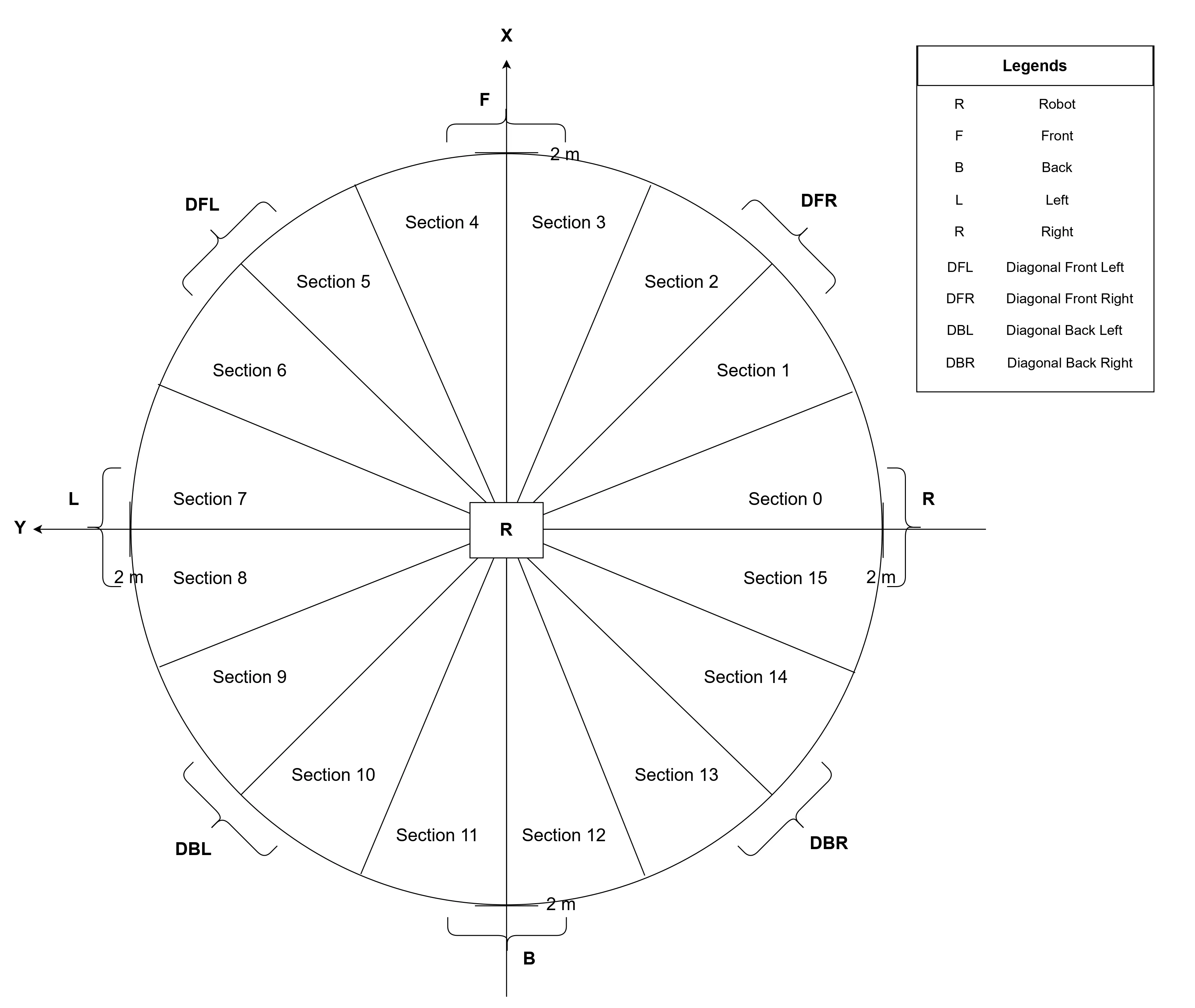
Circular Regions Approach
In addition to previously explained approaches, the circular approach was unique. The circular area of 2m around the robot was divided into 16 equal sections to generate ROIs. The table below exhibits the limits and composition of each ROI.
ROIs |
Section |
Angle |
|---|---|---|
Front |
Section 3 + Section 4 |
67.5° to 112.5° |
Back |
Section 11 + Section 12 |
247.5° to 292.5° |
Left |
Section 7 + Section 8 |
157.5° to 202.5° |
Right |
Section 15 + Section 0 |
337.5° to 360° + 0° to 22.5° |
Diagonal Front Left |
Section 5 + Section 6 |
112.5° to 157.5° |
Diagonal Front Right |
Section 1 + Section 2 |
22.5° to 67.5° |
Diagonal Back Left |
Section 9 + Section 10 |
202.5° to 247.5° |
Diagonal Back Right |
Section 13 + Section 14 |
292.5° to 337.5° |
According to the limits and categorization shown in the table the circular approach can be visualized as in Fig. 3c The figure itself illustrates that it is not a good fit for junction structures due to differences in the shapes of junction structures and approach design. Also, there are not any gaps between ROIs to differentiate between data points. Despite being of its uniqueness the circular approach was not a suitable approach for junction types. There were no gaps between ROIs and also due to the convergence of the circle inwards, ROIs were too close. The data was not logically correct hence resulted in returning false positive results.
3c. Circular Approach
Hybrid Approach
To extract as much information as possible from the surroundings of the robot, A hybrid approach was designed containing appropriate gaps between its ROIs, larger squared diagonal regions to cover maximum area, and thin rectangular areas in front, back, left, and right according to the size of the robot. The limits for the designed hybrid approach are shown in Fig. 3d.
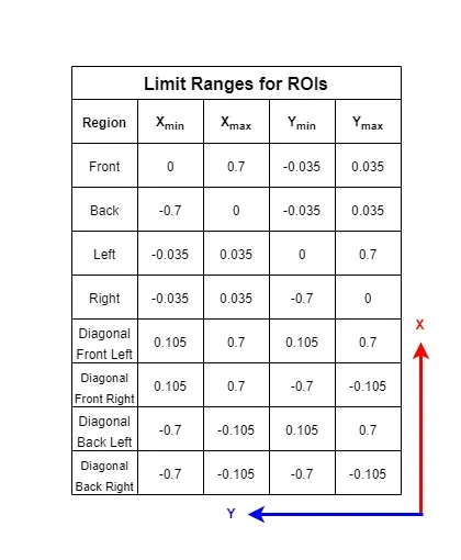
3d. Limit Ranges
According to the limits defined in the table of Fig. 3d the hybrid approach can be envisioned in Fig. 3e. Due to well defined limits of ROIs the hybrid approach proved to be the best fit for the junction types. The points with useful information can easily be retrieved using this approach.
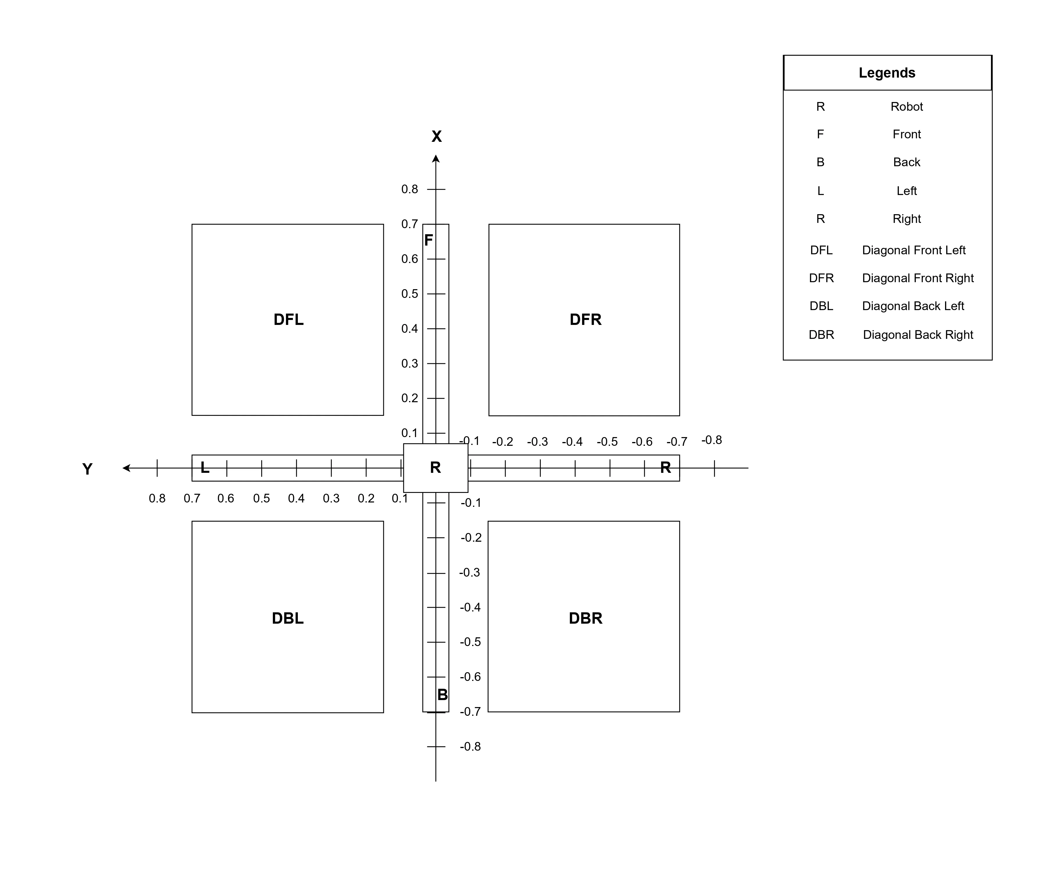
3e. Hybrid Approach
Environment Segmentation Work Flow
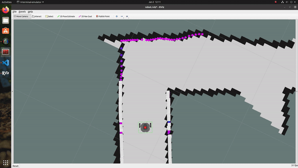
The Junction Synthesizer creates imaginary regions around the robot same as the proposed hybrid approach and then filters and categorizes the lidar points falling into these regions. The Fig. 3f shows an overview of the overall functionality of a junction synthesizer.
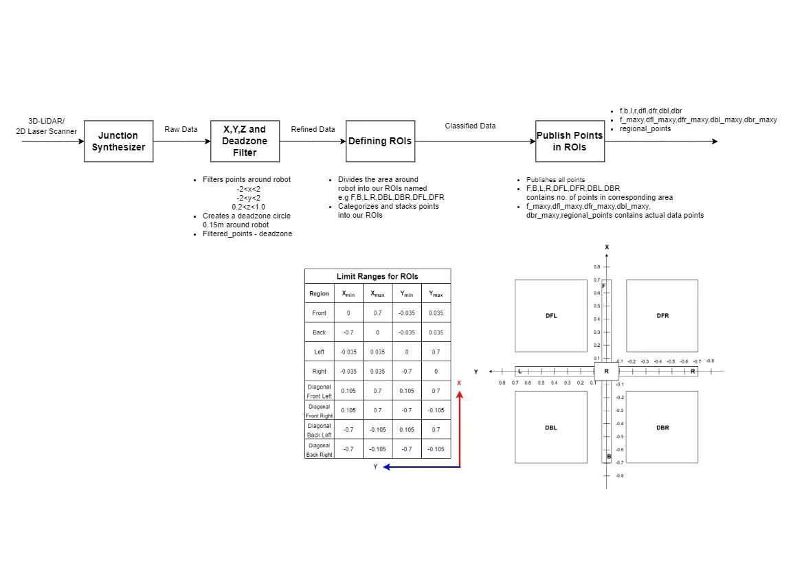
3f. Environment Segmentation Work Flow
Environment Identification
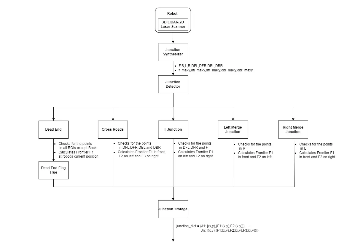
The junction detector plays a crucial role in identifying the robot’s surroundings. It utilizes the data collected by the junction synthesizer’s hybrid approach. Detecting and classifying various junction types such as dead ends, straight paths, cross-road junctions, T-junctions, left merge junctions, and right merge junctions is the main goal. The robot’s ability to navigate and make decisions depends on this data.
Determining and identifying regions of interest (ROIs) within the LIDAR point cloud is a crucial step. These ROIs line up with particular geometric patterns that denote various kinds of junctions. For example, a dead end is identified when lidar data points are present in all ROIs except back. Comparably, when data points are present on both sides left and right but not in the front or rear, a straight path is identified.
Based on the patterns of different junctions and the shape of our hybrid approach a strategy was developed to detect various junctions types and identify their frontiers. The Fig. 4a reveals the strategy for the identification of different junction types and their respective frontiers.
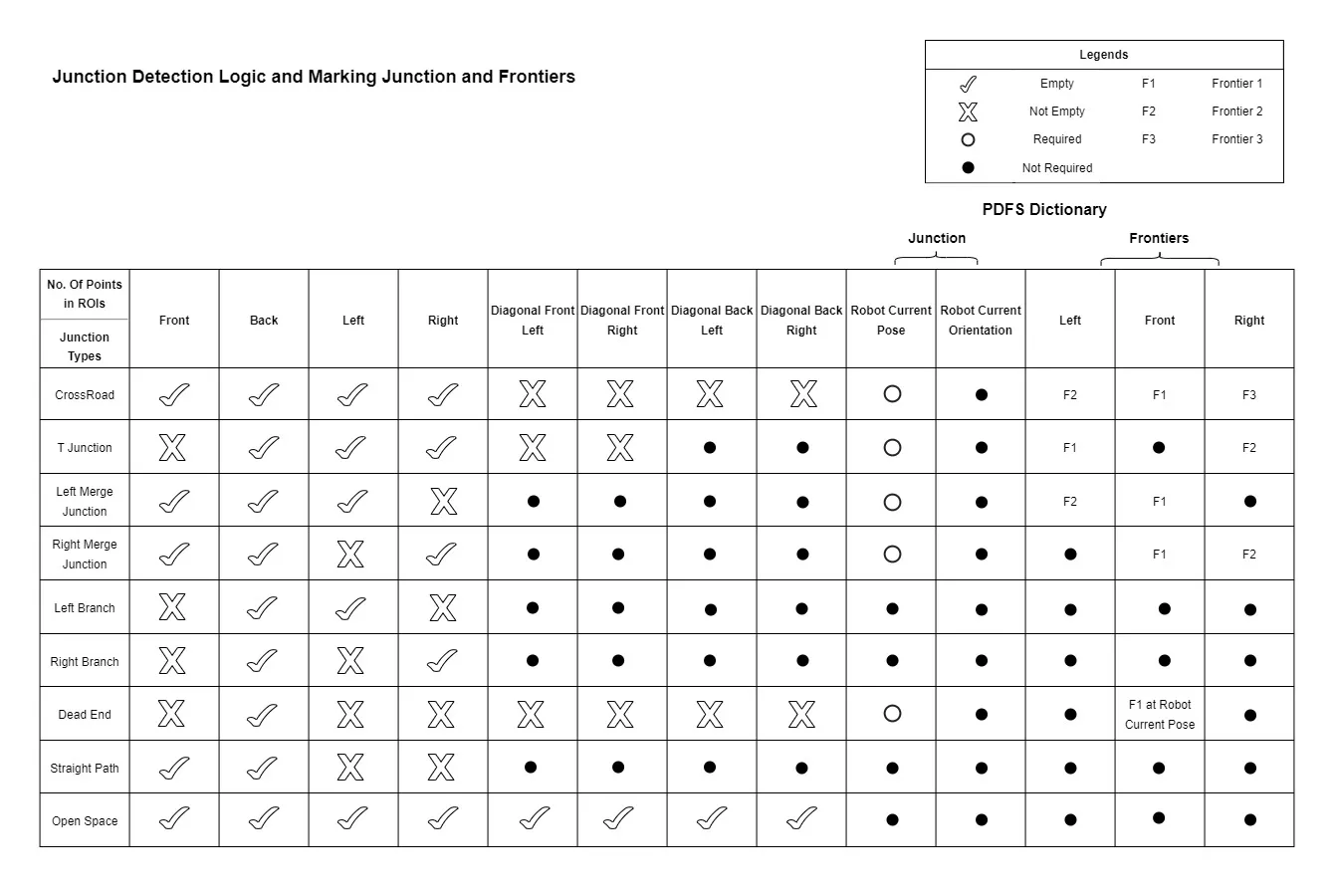
4a. Environment Identification Table
Cross-Road Junction Detection: When LIDAR points are present in every diagonal direction (dfl, dfr, dbl, and dbr) and all cardinal directions (f, b, l, and r) are vacant, a cross-road junction is identified.
T-Junction Detection: When space is occupied in the front (f), diagonal front left (dfl), and diagonal front right (dfr), and there are no points in the back (b), right (r), or left (l) directions, a T-junction is recognized.
Left Merge Junction Detection: Left merge junction is detected when the right (r) side is occupied with points but the rear (b), front (f), and left (l) directions are empty.
Right Merge Junction Detection: A closed left (l) side with no points in the front (f), rear (r), or right (r) directions indicates the presence of a right merge junction.
Left Branch Detection: Left Branch is detected when the right (r) side and front (f) are occupied with points but the back (b), and left (l) directions are empty.
Right Branch Detection: Right Branch is identified when the left (l) side and front (f) are occupied with points but the back (b), and right (r) directions are empty.
Dead End Detection: A dead end is recognized when points are present in the front (f), left (l), right (r), diagonal front left (dfl), diagonal front right (dfr), diagonal back left (dbl), diagonal back right (dbr), directions but not in the back (b) direction.
Straight Path Detection: When points are present on both sides left and right but not in the front (f) and back (b) directions, a straight path is identified.
Open Space Detection: When no points are found in either direction, open space is identified.
Frontiers Calculation
Crossroad, t junction, left merge junction, right merge junction, and dead-end are the cases where there are potential frontiers available for further exploration. In the following sections, the calculation of frontiers in each case is shown.
Frontiers Calculation in CrossRoad Junction Case
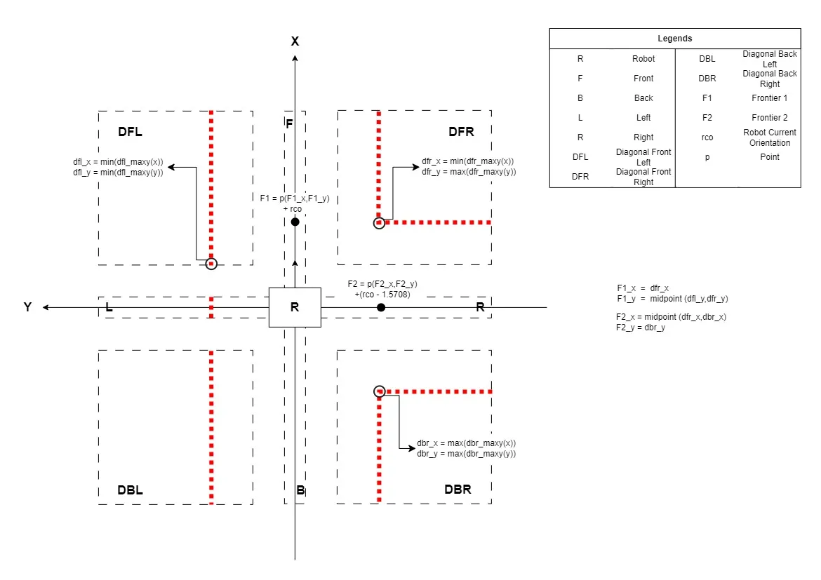
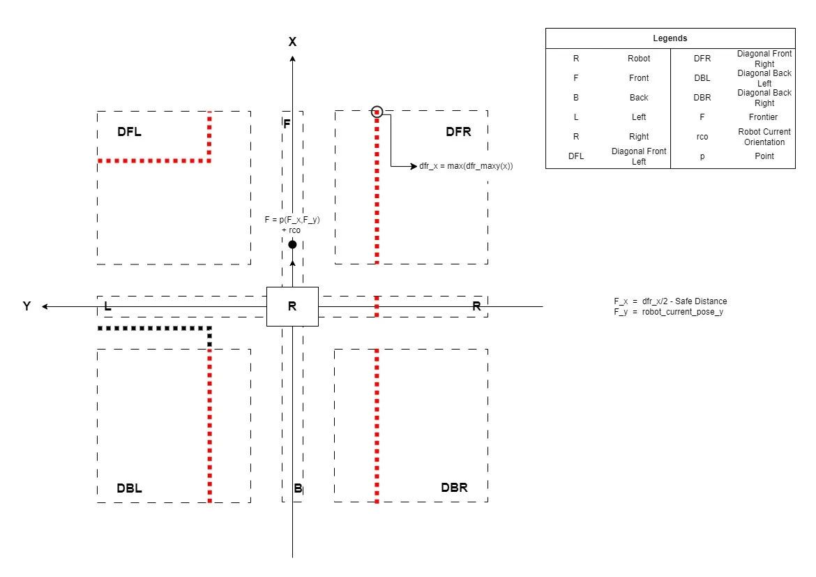
In case of a crossroads junction detection, according to the condition, there should be data points present in all diagonals ROIs. Also, Its detection indicates the presence of three possible ways from here in front, left, and right. As illustrated in the Fig. 4b. To calculate these three potential frontiers the data points from all diagonal ROIs are utilized.
Frontier 1 is calculated by taking a data point from the diagonal front right (containing the minimum value of x and maximum value of y) and a point from the diagonal front left (containing the minimum value of x and minimum value of y). The midpoint of these two points gives us our frontier 1 in front.
Frontier 2 is calculated by taking a data point from the diagonal front left (containing the minimum value of x and minimum value of y) and a point from the diagonal back left (containing the maximum value of x and minimum value of y). The midpoint of these two points gives us our frontier 2 on the left.
Similarly, Frontier 3 is calculated by taking a data point from the diagonal front right (containing minimum value of x and maximum value of y) and a point from the diagonal back right (containing maximum value of x and maximum value of y). The midpoint of these two points gives us our frontier 3 in front.
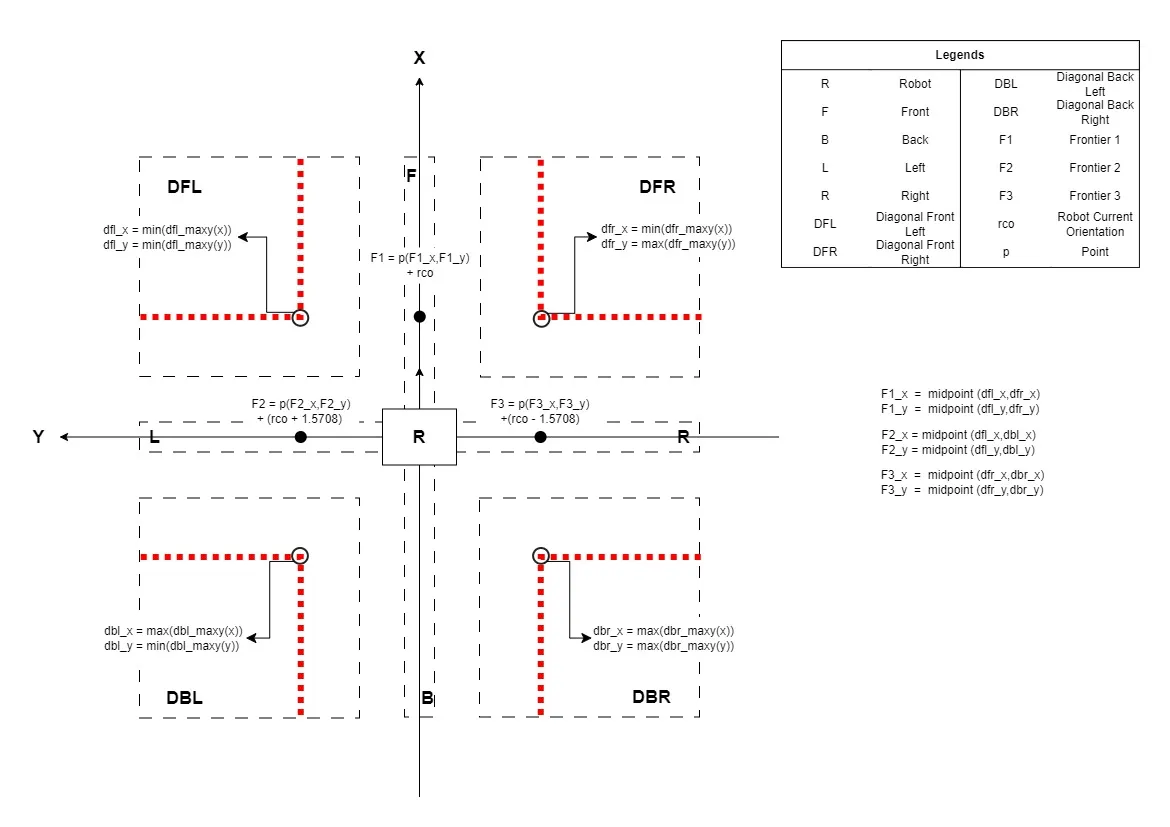
4b. Frontiers Calculation in CrossRoad Junction
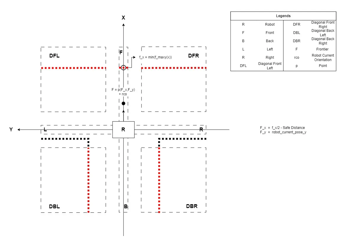
Frontiers Calculation in T Junction Case
In the case of a t junction recognition, all diagonal ROIs and front should contain data points according to the condition. Also, Its detection indicates the presence of two possible ways from here on left and right. To calculate these two potential frontiers the data points from all diagonal ROIs are utilized.
Frontier 1 is calculated by taking a data point from the diagonal front left (containing the minimum value of x ) and a point from the diagonal back left (containing the maximum value of x and minimum value of y). The midpoint of these two points x-coordinate gives us our frontier 1’s x-component and y component is directly taken from the diagonal back left’s y-component on the left.
Frontier 2 is calculated by taking a data point from the diagonal front right (containing the minimum value of x ) and a point from the diagonal back right (containing the maximum value of x and the maximum value of y). The midpoint of these two points x-coordinate gives us our frontier 2’s x-component and the y-component is directly taken from the diagonal back right’s y-component on the right.
The Fig. 4c demonstrates frontiers calculation in case of a T Junction detection.
4c. Frontiers Calculation in T Junction
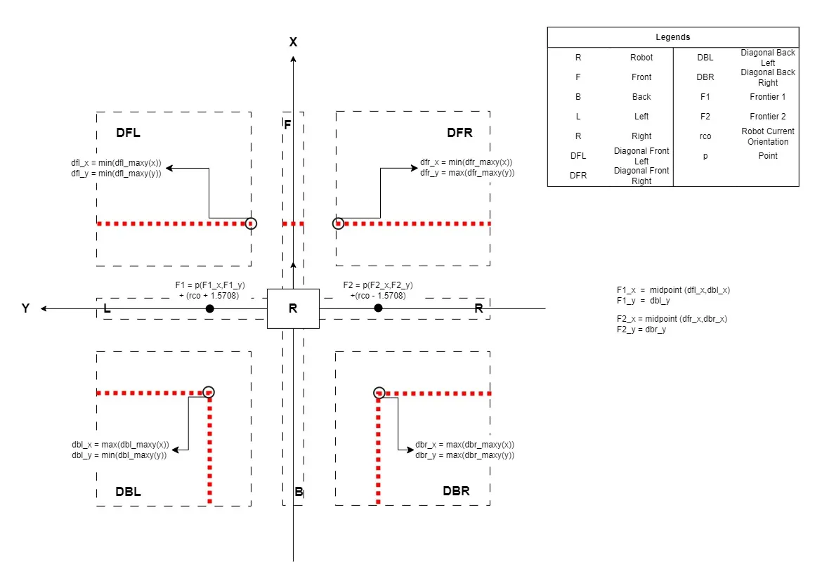
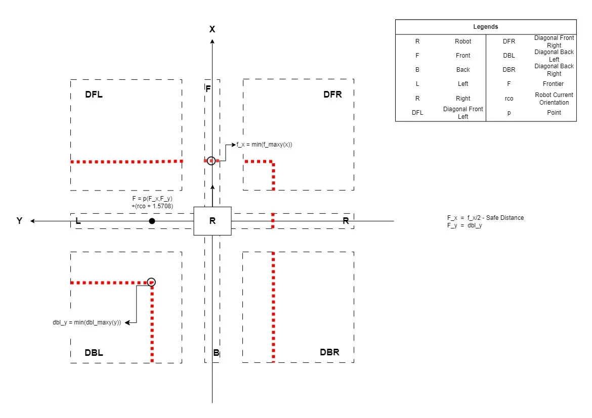
Frontiers Calculation in Left Merge Junction Case
In case of a left merge junction identification, the diagonal front left, diagonal front right, diagonal back left, diagonal back right, and right ROIs should contain data points according to the condition. Also, Its detection indicates the presence of two possible ways from here on the left and in front. To calculate these two potential frontiers the data points from all diagonal ROIs except diagonal back right are utilized. The Fig. 4d exhibits the points of interest and potential frontiers in case of a left merge junction.
Frontier 1 is calculated by taking a data point from the diagonal front right (containing maximum value of y) and a point from the diagonal front left (containing minimum value of x and minimum value of y). The midpoint of these two points y-coordinate gives us our frontier 1’s y-component and the x-component is directly taken from the diagonal front left’s x-component in front.
Frontier 2 is calculated by taking a data point from the diagonal front left (containing minimum value of x ) and a point from the diagonal back left (containing maximum value of x and minimum value of y). The midpoint of these two points’ x-coordinate gives us our frontier 1’s x-component and the y-component is directly taken from the diagonal back left’s y-component on the left.
4d. Frontiers Calculation in Left Merge Junction
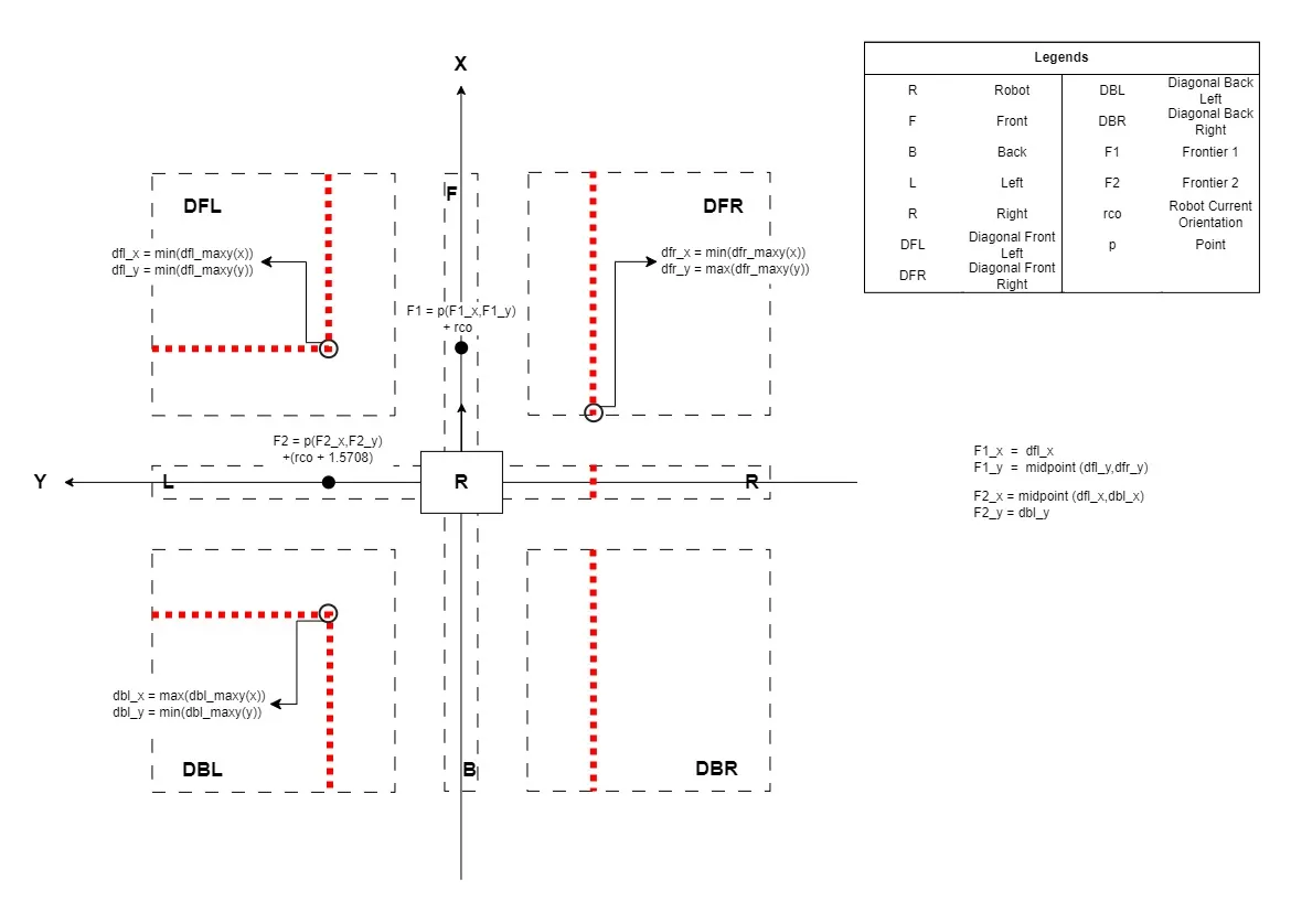
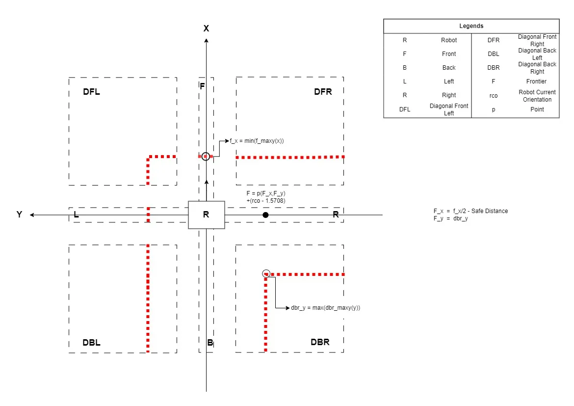
Frontiers Calculation in Right Merge Junction Case
In case of a right merge junction detection, the diagonal front left, diagonal front right, diagonal back left, diagonal back right, and left ROIs should contain data points according to the condition. Also, Its detection indicates the presence of two possible ways from here on the left and front. To calculate these two potential frontiers the data points from all diagonal ROIs except diagonal back right are utilized.
Frontier 1 is calculated by taking a data point from the diagonal front right (containing the minimum value of x and maximum value of y) and a point from the diagonal front left (containing the minimum value of y). The midpoint of these two points y-coordinate gives us our frontier 1’s y-component and the x-component is directly taken from diagonal front right’s x-component in front.
Frontier 2 is calculated by taking a data point from the diagonal front right (containing the minimum value of x) and a point from the diagonal back right (containing the maximum value of x and the maximum value of y). The midpoint of these two points’ x-coordinate gives us our frontier 1’s x-component and the y-component is directly taken from the diagonal back right’s y-component on th4f. Frontiers Calculation in Dead Ende right.
The Fig 4e shows the calculation of potential frontiers in case of right merge junction.
4e. Frontiers Calculation in Right Merge Junction
Frontiers Calculation in Dead End Case
In case of a dead-end detection, All ROIs except the back should contain data points according to the condition. Also, Its detection indicates the presence of only one possible way from here on back. So it marks the robot’s current position as a frontier. The Fig. Junction_detection_de_final.webp depicts the scenario of a dead-end case.
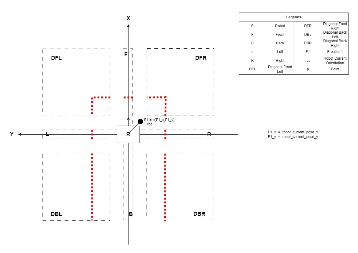
4f. Frontiers Calculation in Dead End
Environment Identification Work Flow
The data supplied by the junction synthesizer gets processed by the junction detector and helps the robot identify its surroundings and navigate through the tunnel. With the help of the data provided by the junction synthesizer, the junction detector identifies different junctions, calculates frontiers according to their type, and saves the information about the junction and its frontiers into a dictionary. An overview of overall functionality is shown in the Fig. 4g. Additionally, in case of a dead-end junction case, it triggers a dead-end flag. Which further utilizes the data stored in the junction dictionary to navigate further(Details of it can be read in section pdfs}).
4g. Environment Identification Work Flow
Autonomous Exploration
Similar to the junction detector, Autonomous exploration also utilizes the data provided by the junction synthesizer to make the robot able to navigate through the tunnel autonomously. Moreover, it has a priority-based depth-first search algorithm which helps the robot to relocate in case of a dead end to continue exploration. An overview of the autonomous exploration node is illustrated in Fig. 5a.
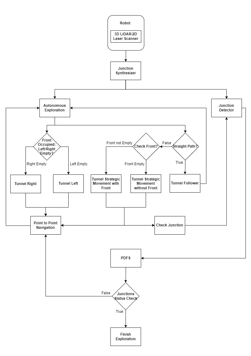
5a. Autonomous Exploration Overview
Case - I Straight Path
The Autonomous exploration node continuously checks for the condition of a straight path i.e. Front should be empty and the left and right should be occupied (see junction detection logic table in Fig. ref{fig: ch4f18}). If the condition satisfies it keeps the robot moving in the forward direction and tries to keep it in the center of the branch. The robot keeps moving in a straight path until the condition fails.
Case - II Strategic Movement
Strategic movement is responsible for bringing the robot a bit forward to have a better understanding of the robot’s surroundings, in case of straight path failure. If the condition for straight path fails then the robot executes strategic movement which is further divided into two cases which are Strategic movement with front and strategic movement without front.
Navigation Goals in Strategic Movement without front Case
Strategic movement without a front case is specially made to deal with the case of left merge junction and right merge junction. The left merge junction and right merge junction are the cases in which the robot doesn’t have points available on the front and it helps the robot to bring it a little bit forward by utilizing the data available in diagonal ROIs. The Fig. 5b shows an example of strategic movement without a front.
5b. Navigation Goals in Strategic Movement without front
As it can be seen in Fig. strategic_movement_without_front _final.webp the Frontier’s x component is calculated by taking a data point from the diagonal front right (maximum value of x), then dividing it into half and subtracting a safe distance and y-component is taken from robots current pose.
Similarly in the case of the right merge junction the Frontier’s x component is calculated by taking a data point from the diagonal front left (maximum value of x), then dividing it into half and subtracting a safe distance, and the y-component is taken from the robot’s current pose.
Navigation Goals in Strategic Movement with front Case
Strategic movement with the front case is designed to deal with the case of T junction and Dead end. The T junction and Dead end are the cases in which the robot has points available on the front and it helps the robot to bring it a little bit forward by utilizing the data available on front ROI. The Fig. 5c shows an example of strategic movement with the front.
5c. Navigation Goals in Strategic Movement with front
As can be seen in the figure the Frontier’s x component is calculated by taking a data point from the front, then dividing it into half and subtracting a safe distance, and the y-component is taken from the robot’s current pose.
Similarly, in the case of a dead end the Frontier’s x component is calculated by taking a data point from the front, then dividing it into half and subtracting a safe distance, and the y-component is taken from the robot’s current pose.
Case - III Branch
Strategic movement is responsible for bringing the robot a bit forward into the branch, in the case of the left/right branch. If the condition for the left/right branch is fulfilled then the robot executes branched case movement which is further divided into two cases which are the left branch case and the right branch case.
Navigation Goals in Left Branch Case
The left branch case is specially made to deal with the case of the left branch. The left branch case helps the robot to bring it a little bit forward into the branch by utilizing the data available in the front ROI. The Fig. 5d shows an example of left branch movement.
5d. Navigation Goals in Left Branch
The Frontier’s x component is calculated by taking a data point from the front, then dividing it into half and subtracting a safe distance, and the y-component is calculated by taking a data point from the diagonal back left (containing the minimum value of y).
Navigation Goals in Right Branch Case
The right branch case is specially made to deal with the case of the right branch. The right branch case helps the robot to bring it a little bit forward into the branch by utilizing the data available in the front ROI. The Fig. 5e shows an example of the right branch movement.
5e. Navigation Goals in Right Branch
The Frontier’s x component is calculated by taking a data point from the front, then dividing it into half and subtracting a safe distance, and the y-component is calculated by taking a data point from the diagonal back right(containing the maximum value of y).